The order of transformation of graphs of functions. Transformation of Graphs of Elementary Functions

Hypothesis: If you study the movement of the graph during the formation of the equation of functions, then you can see that all graphs obey general patterns therefore, it is possible to formulate general laws regardless of the functions, which will not only facilitate the construction of graphs various functions but also use them in problem solving.

Purpose: To study the movement of graphs of functions:

1) The task of studying literature

2) Learn to build graphs of various functions

3) Learn how to convert charts linear functions

4) Consider the use of graphs in solving problems

Object of study: Graphs of functions

Subject of research: Movements of graphs of functions

Relevance: The construction of function graphs, as a rule, takes a lot of time and requires attention from the student, but knowing the rules for transforming function graphs and graphs of basic functions, you can quickly and easily build function graphs, which will allow you not only to complete tasks for plotting function graphs, but also solve related problems (to find the maximum (minimum height of time and meeting point))

This project is useful to all students of the school.

Literature review:

The literature discusses ways to construct a graph of various functions, as well as examples of the transformation of graphs of these functions. Graphs of almost all the main functions are used in various technical processes, which allows you to more clearly present the course of the process and program the result

Permanent function. This function is given by the formula y = b, where b is some number. The graph of a constant function is a straight line parallel to the x-axis and passing through the point (0; b) on the y-axis. The graph of the function y \u003d 0 is the abscissa axis.

Types of function 1Direct proportionality. This function is given by the formula y \u003d kx, where the coefficient of proportionality k ≠ 0. The direct proportionality graph is a straight line passing through the origin.

Linear function. Such a function is given by the formula y = kx + b, where k and b are real numbers. The graph of a linear function is a straight line.

Linear function graphs can intersect or be parallel.

So, the lines of the graphs of linear functions y \u003d k 1 x + b 1 and y \u003d k 2 x + b 2 intersect if k 1 ≠ k 2; if k 1 = k 2 , then the lines are parallel.

2 Inverse proportionality is a function that is given by the formula y \u003d k / x, where k ≠ 0. K is called the coefficient inverse proportionality. The inverse proportionality graph is a hyperbola.

The function y \u003d x 2 is represented by a graph called a parabola: on the interval [-~; 0] the function is decreasing, on the interval the function is increasing.

The function y \u003d x 3 increases along the entire number line and is graphically represented by a cubic parabola.

Power function with natural exponent. This function is given by the formula y \u003d x n, where n is natural number. Graphs power function with a natural exponent depend on n. For example, if n = 1, then the graph will be a straight line (y = x), if n = 2, then the graph will be a parabola, etc.

A power function with a negative integer exponent is represented by the formula y \u003d x -n, where n is a natural number. This function is defined for all x ≠ 0. The graph of the function also depends on the exponent n.

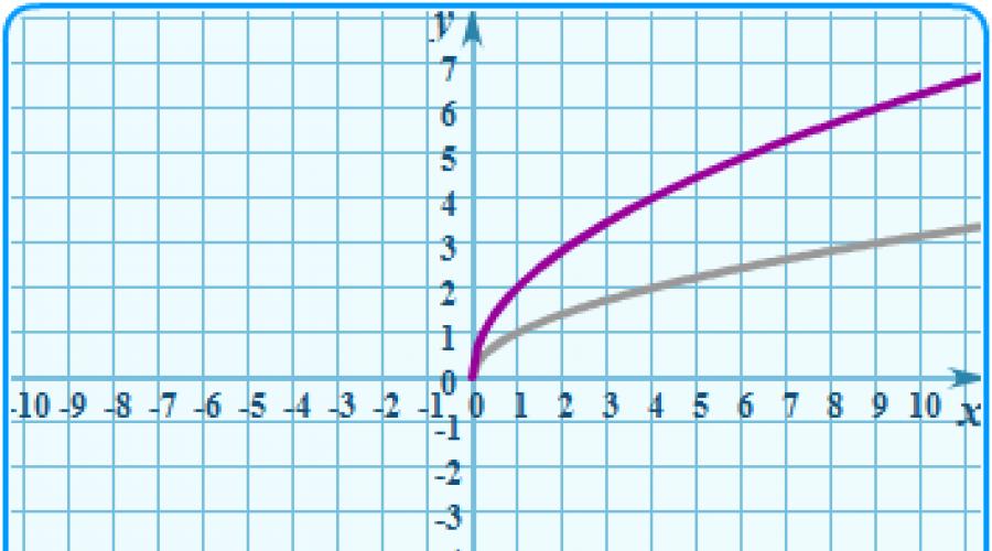
Power function with a positive fractional exponent. This function is represented by the formula y \u003d x r, where r is a positive irreducible fraction. This function is also neither even nor odd.

Graph-line that displays the relationship of dependent and independent variables on the coordinate plane. The graph serves to visually display these elements.

An independent variable is a variable that can take on any value in the scope of a function (where given function makes sense (can't divide by zero)

To plot a function graph,

1) Find ODZ (range of acceptable values)

2) take some arbitrary values ​​for the independent variable

3) Find the value of the dependent variable

4) Build a coordinate plane, mark these points on it

5) Connect their lines if necessary, explore the resulting graph Converting graphs elementary functions.

Graph Conversion

IN pure form the basic elementary functions are encountered, unfortunately, not so often. Much more often one has to deal with elementary functions obtained from basic elementary functions by adding constants and coefficients. Graphs of such functions can be built by applying geometric transformations to the graphs of the corresponding basic elementary functions (or by switching to a new coordinate system). Eg, quadratic function the formula is a quadratic parabola formula, compressed three times relative to the ordinate axis, symmetrically displayed relative to the abscissa axis, shifted against the direction of this axis by 2/3 units and shifted along the direction of the ordinate axis by 2 units.

Let's understand these geometric transformations of a function graph step by step using specific examples.

With the help of geometric transformations of the graph of the function f (x), a graph of any function of the form formula can be constructed, where the formula is the compression or expansion coefficients along the oy and ox axes, respectively, the minus signs in front of the coefficients formula and formula indicate a symmetrical display of the graph with respect to coordinate axes, a and b define the shift relative to the abscissa and ordinate axes, respectively.

Thus, there are three types of geometric transformations of the function graph:

The first type is scaling (compression or expansion) along the abscissa and ordinate axes.

The need for scaling is indicated by formula coefficients other than one, if the number is less than 1, then the graph is compressed relative to oy and stretched relative to ox, if the number is greater than 1, then we stretch along the ordinate axis and shrink along the abscissa axis.

The second type is a symmetrical (mirror) display with respect to the coordinate axes.

The need for this transformation is indicated by the minus signs in front of the coefficients of the formula (in this case, we display the graph symmetrically with respect to the ox axis) and the formula (in this case, we display the graph symmetrically with respect to the y axis). If there are no minus signs, then this step is skipped.

Parallel transfer.

TRANSFER ALONG THE Y-AXIS

f(x) => f(x) - b
Let it be required to plot the function y \u003d f (x) - b. It is easy to see that the ordinates of this graph for all values ​​of x on |b| units less than the corresponding ordinates of the graph of functions y = f(x) for b>0 and |b| more units - at b 0 or up at b To plot the function y + b = f(x), plot the function y = f(x) and move the x-axis to |b| units up for b>0 or by |b| units down at b

TRANSFER ALONG THE X-AXIS

f(x) => f(x + a)
Let it be required to plot the function y = f(x + a). Consider a function y = f(x), which at some point x = x1 takes the value y1 = f(x1). Obviously, the function y = f(x + a) will take the same value at the point x2, the coordinate of which is determined from the equality x2 + a = x1, i.e. x2 = x1 - a, and the equality under consideration is valid for the totality of all values ​​from the domain of the function. Therefore, the graph of the function y = f(x + a) can be obtained by parallel displacement of the graph of the function y = f(x) along the x-axis to the left by |a| ones for a > 0 or to the right by |a| units for a To plot the function y = f(x + a), plot the function y = f(x) and move the y-axis to |a| units to the right for a>0 or |a| units to the left for a

Examples:

1.y=f(x+a)

2.y=f(x)+b

Reflection.

GRAPHING OF A FUNCTION OF THE VIEW Y = F(-X)

f(x) => f(-x)
Obviously, the functions y = f(-x) and y = f(x) take equal values ​​at points whose abscissas are equal in absolute value, but opposite in sign. In other words, the ordinates of the graph of the function y = f(-x) in the region of positive (negative) values ​​of x will be equal to the ordinates of the graph of the function y = f(x) with negative (positive) x values ​​corresponding in absolute value. Thus, we get the following rule.
To plot the function y = f(-x), you should plot the function y = f(x) and reflect it along the y-axis. The resulting graph is the graph of the function y = f(-x)

GRAPHING OF A FUNCTION OF THE VIEW Y = - F(X)

f(x) => - f(x)
The ordinates of the graph of the function y = - f(x) for all values ​​of the argument are equal in absolute value, but opposite in sign to the ordinates of the graph of the function y = f(x) for the same values ​​of the argument. Thus, we get the following rule.
To plot the function y = - f(x), you should plot the function y = f(x) and reflect it about the x-axis.

Examples:

1.y=-f(x)

2.y=f(-x)

3.y=-f(-x)

Deformation.

DEFORMATION OF THE GRAPH ALONG THE Y-AXIS

f(x) => kf(x)
Consider a function of the form y = k f(x), where k > 0. It is easy to see that for equal values ​​of the argument, the ordinates of the graph of this function will be k times greater than the ordinates of the graph of the function y = f(x) for k > 1 or 1/k times less than the ordinates of the graph of the function y = f(x) for k ) or decrease its ordinates by 1/k times for k
k > 1- stretching from the Ox axis
0 - compression to the OX axis

GRAPH DEFORMATION ALONG THE X-AXIS

f(x) => f(kx)
Let it be required to plot the function y = f(kx), where k>0. Consider a function y = f(x), which takes the value y1 = f(x1) at an arbitrary point x = x1. It is obvious that the function y = f(kx) takes the same value at the point x = x2, the coordinate of which is determined by the equality x1 = kx2, and this equality is valid for the totality of all values ​​of x from the domain of the function. Consequently, the graph of the function y = f(kx) is compressed (for k 1) along the abscissa axis relative to the graph of the function y = f(x). Thus, we get the rule.
To plot the function y = f(kx), plot the function y = f(x) and reduce its abscissas by k times for k>1 (compress the graph along the abscissa axis) or increase its abscissas by 1/k times for k
k > 1- compression to the Oy axis
0 - stretching from the OY axis

Depending on the conditions of the course of physical processes, some quantities take constant values ​​and are called constants, others change under certain conditions and are called variables.

careful study environment shows that physical quantities are dependent on each other, that is, a change in some quantities entails a change in others.

Mathematical analysis studies the quantitative relationships of mutually changing quantities, abstracting from the specific physical meaning. One of the basic concepts of mathematical analysis is the concept of a function.

Consider the elements of the set and the elements of the set
(Fig. 3.1).

If some correspondence is established between the elements of the sets
And as a rule , then we note that the function is defined
.

Definition 3.1. Correspondence , which is associated with each element not an empty set
some well-defined element not an empty set , is called a function or mapping
V .

Symbolically display
V is written as follows:

.

At the same time, many
is called the domain of the function and is denoted
.

In turn, many is called the range of the function and is denoted
.

In addition, it should be noted that the elements of the set
are called independent variables, the elements of the set are called dependent variables.

Ways to set a function

The function can be defined in the following main ways: tabular, graphical, analytical.

If, on the basis of experimental data, tables are compiled that contain the values ​​of the function and the corresponding values ​​of the argument, then this method of specifying the function is called tabular.

At the same time, if some studies of the result of the experiment are output to the registrar (oscilloscope, recorder, etc.), then it is noted that the function is set graphically.

The most common is the analytical way of defining a function, i.e. a method in which the independent and dependent variables are linked using a formula. Wherein essential role plays the scope of the function:

different, although they are given by the same analytical relations.

If only the function formula is given
, then we consider that the domain of definition of this function coincides with the set of those values ​​of the variable , for which the expression
has the meaning. In this regard, the problem of finding the domain of a function plays a special role.

Task 3.1. Find the scope of a function

Solution

The first term takes real values ​​at
, and the second at. Thus, to find the domain of definition given function it is necessary to solve the system of inequalities:

As a result of the solution of such a system, we obtain . Therefore, the domain of the function is the segment
.

The simplest transformations of graphs of functions

The construction of graphs of functions can be greatly simplified if we use the known graphs of the main elementary functions. The following functions are called basic elementary functions:

1) power function
Where
;

2) exponential function
Where
And
;

3) logarithmic function
, Where - any positive number other than one:
And
;

4) trigonometric functions




;
.

5) inverse trigonometric functions
;
;
;
.

Elementary functions are called functions that are obtained from basic elementary functions using four arithmetic operations and superpositions applied a finite number of times.

Simple geometric transformations also simplify the process of plotting functions. These transformations are based on the following statements:

The graph of the function y=f(x+a) is the graph y=f(x), shifted (for a >0 to the left, for a< 0 вправо) на |a| единиц параллельно осиOx.

Graph of the function y=f(x) +b has graphs y=f(x), shifted (if b>0 up, if b< 0 вниз) на |b| единиц параллельно осиOy.

The graph of the function y = mf(x) (m0) is the graph y = f(x), stretched (for m>1) m times or compressed (for 0

The graph of the function y = f(kx) is the graph y = f(x), compressed (for k > 1) k times or stretched (for 0< k < 1) вдоль оси Ox. При –< k < 0 график функции y = f(kx) есть зеркальное отображение графика y = f(–kx) от оси Oy.