Which function is called even and odd. Function study

Evenness and oddness of a function are one of its main properties, and parity takes up an impressive part school course mathematics. It largely determines the behavior of the function and greatly facilitates the construction of the corresponding graph.

Let's determine the parity of the function. Generally speaking, the function under study is considered even if for opposite values ​​of the independent variable (x) located in its domain of definition, the corresponding values ​​of y (function) turn out to be equal.

Let's give a more strict definition. Consider some function f (x), which is defined in the domain D. It will be even if for any point x located in the domain of definition:

• -x (opposite point) also lies in this scope,

• f(-x) = f(x).

From the above definition follows the condition necessary for the domain of definition of such a function, namely, symmetry with respect to the point O, which is the origin of coordinates, since if some point b is contained in the domain of definition of an even function, then the corresponding point b also lies in this domain. From the above, therefore, the conclusion follows: even function has a symmetrical appearance with respect to the ordinate axis (Oy).

How to determine the parity of a function in practice?

Let it be specified using the formula h(x)=11^x+11^(-x). Following the algorithm that follows directly from the definition, we first examine its domain of definition. Obviously, it is defined for all values ​​of the argument, that is, the first condition is met.

The next step is to substitute the opposite value (-x) for the argument (x).
We get:
h(-x) = 11^(-x) + 11^x.
Since addition satisfies the commutative (commutative) law, it is obvious that h(-x) = h(x) and the given functional dependence- even.

Let's check the parity of the function h(x)=11^x-11^(-x). Following the same algorithm, we get that h(-x) = 11^(-x) -11^x. Taking out the minus, in the end we have
h(-x)=-(11^x-11^(-x))=- h(x). Therefore, h(x) is odd.

By the way, it should be recalled that there are functions that cannot be classified according to these criteria; they are called neither even nor odd.

Even functions have a number of interesting properties:

• as a result of adding similar functions, they get an even one;
• as a result of subtracting such functions, an even one is obtained;
• even, also even;
• as a result of multiplying two such functions, an even one is obtained;
• as a result of multiplying odd and even functions, an odd one is obtained;
• as a result of dividing odd and even functions, an odd one is obtained;
• the derivative of such a function is odd;
• If you square an odd function, you get an even one.

The parity of a function can be used to solve equations.

To solve an equation like g(x) = 0, where left side equation is an even function, it will be quite enough to find its solutions for non-negative values ​​of the variable. The resulting roots of the equation must be combined with the opposite numbers. One of them is subject to verification.

This is also successfully used to solve non-standard tasks with parameter.

For example, is there any value of the parameter a for which the equation 2x^6-x^4-ax^2=1 will have three roots?

If we take into account that the variable enters the equation in even powers, then it is clear that replacing x with - x given equation won't change. It follows that if a certain number is its root, then the opposite number is also the root. The conclusion is obvious: the roots of an equation that are different from zero are included in the set of its solutions in “pairs”.

It is clear that the number itself is not 0, that is, the number of roots of such an equation can only be even and, naturally, for any value of the parameter it cannot have three roots.

But the number of roots of the equation 2^x+ 2^(-x)=ax^4+2x^2+2 can be odd, and for any value of the parameter. Indeed, it is easy to check that the set of roots of this equation contains solutions “in pairs”. Let's check if 0 is a root. When we substitute it into the equation, we get 2=2. Thus, in addition to “paired” ones, 0 is also a root, which proves their odd number.

Even function.

Even is a function whose sign does not change when the sign changes x.

x equality holds f(–x) = f(x). Sign x does not affect the sign y.

The graph of an even function is symmetrical about the coordinate axis (Fig. 1).

Examples of an even function:

y=cos x

y = x 2

y = –x 2

y = x 4

y = x 6

y = x 2 + x

Explanation:
Let's take the function y = x 2 or y = –x 2 .
For any value x the function is positive. Sign x does not affect the sign y. The graph is symmetrical about the coordinate axis. This is an even function.

Odd function.

Odd is a function whose sign changes when the sign changes x.

In other words, for any value x equality holds f(–x) = –f(x).

The graph of an odd function is symmetrical with respect to the origin (Fig. 2).

Examples of odd function:

y= sin x

y = x 3

y = –x 3

Explanation:

Let's take the function y = – x 3 .
All meanings at it will have a minus sign. That is a sign x influences the sign y. If the independent variable is a positive number, then the function is positive, if the independent variable is a negative number, then the function is negative: f(–x) = –f(x).
The graph of the function is symmetrical about the origin. This is an odd function.

Properties of even and odd functions:

NOTE:

Not all functions are even or odd. There are functions that do not obey such gradation. For example, the root function at = √X does not apply to either even or odd functions (Fig. 3). When listing the properties of such functions, an appropriate description should be given: neither even nor odd.

Periodic functions.

As you know, periodicity is the repetition of certain processes at a certain interval. The functions that describe these processes are called periodic functions. That is, these are functions in whose graphs there are elements that repeat at certain numerical intervals.

A function is called even (odd) if for any and the equality

.

The graph of an even function is symmetrical about the axis
.

The graph of an odd function is symmetrical about the origin.

Example 6.2. Examine whether a function is even or odd

1)
; 2)
; 3)
.

Solution.

1) The function is defined when
. We'll find
.

Those.
. Means, this function is even.

2) The function is defined when

Those.
. Thus, this function is odd.

3) the function is defined for , i.e. For

,
. Therefore the function is neither even nor odd. Let's call it a function of general form.

3. Study of the function for monotonicity.

Function
is called increasing (decreasing) on ​​a certain interval if in this interval each higher value argument corresponds to a larger (smaller) value of the function.

Functions increasing (decreasing) over a certain interval are called monotonic.

If the function
differentiable on the interval
and has a positive (negative) derivative
, then the function
increases (decreases) over this interval.

Example 6.3. Find intervals of monotonicity of functions

1)
; 3)
.

Solution.

1) This function is defined on the entire number line. Let's find the derivative.

The derivative is equal to zero if
And
. The domain of definition is the number axis, divided by dots
,
at intervals. Let us determine the sign of the derivative in each interval.

In the interval
the derivative is negative, the function decreases on this interval.

In the interval
the derivative is positive, therefore, the function increases over this interval.

2) This function is defined if
or

.

We determine the sign of the quadratic trinomial in each interval.

Thus, the domain of definition of the function

Let's find the derivative
,
, If
, i.e.
, But
. Let us determine the sign of the derivative in the intervals
.

In the interval
the derivative is negative, therefore, the function decreases on the interval
. In the interval
the derivative is positive, the function increases over the interval
.

4. Study of the function at the extremum.

Dot
called the maximum (minimum) point of the function
, if there is such a neighborhood of the point that's for everyone
from this neighborhood the inequality holds

.

The maximum and minimum points of a function are called extremum points.

If the function
at the point has an extremum, then the derivative of the function at this point is equal to zero or does not exist (a necessary condition for the existence of an extremum).

The points at which the derivative is zero or does not exist are called critical.

5. Sufficient conditions for the existence of an extremum.

Rule 1. If during the transition (from left to right) through the critical point derivative
changes sign from “+” to “–”, then at the point function
has a maximum; if from “–” to “+”, then the minimum; If
does not change sign, then there is no extremum.

Rule 2. Let at the point
first derivative of a function
equal to zero
, and the second derivative exists and is different from zero. If
, That – maximum point, if
, That – minimum point of the function.

Example 6.4 . Explore the maximum and minimum functions:

1)
; 2)
; 3)
;

4)
.

Solution.

1) The function is defined and continuous on the interval
.

Let's find the derivative
and solve the equation
, i.e.
.From here
– critical points.

Let us determine the sign of the derivative in the intervals ,
.

When passing through points
And
the derivative changes sign from “–” to “+”, therefore, according to rule 1
– minimum points.

When passing through a point
the derivative changes sign from “+” to “–”, so
– maximum point.

,
.

2) The function is defined and continuous in the interval
. Let's find the derivative
.

Having solved the equation
, we'll find
And
– critical points. If the denominator
, i.e.
, then the derivative does not exist. So,
– third critical point. Let us determine the sign of the derivative in intervals.

Therefore, the function has a minimum at the point
, maximum in points
And
.

3) A function is defined and continuous if
, i.e. at
.

Let's find the derivative

.

Let's find critical points:

Neighborhoods of points
do not belong to the domain of definition, therefore they are not extrema. So, let's examine the critical points
And
.

4) The function is defined and continuous on the interval
. Let's use rule 2. Find the derivative
.

Let's find critical points:

Let's find the second derivative
and determine its sign at the points

At points
function has a minimum.

At points
the function has a maximum.

Graphs of even and odd functions have the following features:

If a function is even, then its graph is symmetrical about the ordinate. If a function is odd, then its graph is symmetrical about the origin.

Solution. Consider the function: \(f\left(x \right)=\left|x \right|\) and substitute the opposite \(-x \) instead of \(x \). As a result of simple transformations we get: $$f\left(-x \right)=\left|-x \right|=\left|x \right|=f\left(x \right)$$ In other words, if replace the argument with the opposite sign, the function will not change.

This means that this function is even, and its graph will be symmetrical with respect to the ordinate axis ( vertical axis). The graph of this function is shown in the figure on the left. This means that when constructing a graph, you can only draw half, and the second part (to the left of the vertical axis, draw symmetrically to the right part). By determining the symmetry of a function before starting to plot its graph, you can greatly simplify the process of constructing or studying the function. If it is difficult to perform a general check, you can do it simpler: substitute the same values ​​of different signs into the equation. For example -5 and 5. If the function values ​​turn out to be the same, then we can hope that the function will be even. From a mathematical point of view, this approach is not entirely correct, but from a practical point of view it is convenient. To increase the reliability of the result, you can substitute several pairs of such opposite values.

Solution. Let's check the same as in the previous example: $$f\left(-x \right)=x\left|-x \right|=-x\left|x \right|=-f\left(x \right) $$ This means that the original function is odd (the sign of the function has changed to the opposite).

Conclusion: the function is symmetrical about the origin. You can build only one half, and draw the second symmetrically. This kind of symmetry is more difficult to draw. This means that you are looking at the chart from the other side of the sheet, and even upside down. Or you can do this: take the drawn part and rotate it around the origin 180 degrees counterclockwise.

Solution. Let's perform the same check for sign change as in the previous two examples. $$f\left(-x \right)=\left(-x \right)^3+\left(-x \right)^2=-x^2+x^2$$ As a result, we get that: $$f\left(-x \right)\not=f\left(x \right),f\left(-x \right)\not=-f\left(x \right)$$ And this means, that the function is neither even nor odd.

Conclusion: the function is not symmetrical either with respect to the origin or the center of the coordinate system. This happened because it is the sum of two functions: even and odd. The same situation will happen if you subtract two different functions. But multiplication or division will lead to a different result. For example, the product of an even and an odd function produces an odd function. Or the quotient of two odd numbers leads to an even function.

Hide Show

Methods for specifying a function

Let the function be given by the formula: y=2x^(2)-3. By assigning any values ​​to the independent variable x, you can calculate, using this formula, the corresponding values ​​of the dependent variable y. For example, if x=-0.5, then, using the formula, we find that the corresponding value of y is y=2 \cdot (-0.5)^(2)-3=-2.5.

Taking any value taken by the argument x in the formula y=2x^(2)-3, you can calculate only one value of the function that corresponds to it. The function can be represented as a table:

Using this table, you can see that for the argument value −1 the function value −3 will correspond; and the value x=2 will correspond to y=0, etc. It is also important to know that each argument value in the table corresponds to only one function value.

More functions can be specified using graphs. Using a graph, it is established which value of the function correlates with a certain value x. Most often, this will be an approximate value of the function.

Even and odd function

The function is even function, when f(-x)=f(x) for any x from the domain of definition. Such a function will be symmetrical about the Oy axis.

The function is odd function, when f(-x)=-f(x) for any x from the domain of definition. Such a function will be symmetric about the origin O (0;0) .

The function is not even, neither odd and is called function general view , when it does not have symmetry about the axis or origin.

Let us examine the following function for parity:

f(x)=3x^(3)-7x^(7)

D(f)=(-\infty ; +\infty) with a symmetric domain of definition relative to the origin. f(-x)= 3 \cdot (-x)^(3)-7 \cdot (-x)^(7)= -3x^(3)+7x^(7)= -(3x^(3)-7x^(7))= -f(x).

This means that the function f(x)=3x^(3)-7x^(7) is odd.

Periodic function

The function y=f(x) , in the domain of which the equality f(x+T)=f(x-T)=f(x) holds for any x, is called periodic function with period T \neq 0 .

Repeating the graph of a function on any segment of the x-axis that has length T.

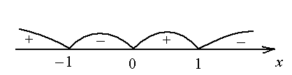
The intervals where the function is positive, that is, f(x) > 0, are segments of the abscissa axis that correspond to the points of the function graph lying above the abscissa axis.

f(x) > 0 on (x_(1); x_(2)) \cup (x_(3); +\infty)

Intervals where the function is negative, that is, f(x)< 0 - отрезки оси абсцисс, которые отвечают точкам графика функции, лежащих ниже оси абсцисс.

f(x)< 0 на (-\infty; x_(1)) \cup (x_(2); x_(3))

Limited function

Bounded from below It is customary to call a function y=f(x), x \in X when there is a number A for which the inequality f(x) \geq A holds for any x \in X .

An example of a function bounded from below: y=\sqrt(1+x^(2)) since y=\sqrt(1+x^(2)) \geq 1 for any x .

Bounded from above a function y=f(x), x \in X is called when there is a number B for which the inequality f(x) \neq B holds for any x \in X .

An example of a function bounded below: y=\sqrt(1-x^(2)), x \in [-1;1] since y=\sqrt(1+x^(2)) \neq 1 for any x \in [-1;1] .

Limited It is customary to call a function y=f(x), x \in X when there is a number K > 0 for which the inequality \left | f(x)\right | \neq K for any x \in X .

Example limited function: y=\sin x is limited on the entire number axis, since \left | \sin x \right | \neq 1.

Increasing and decreasing function

It is customary to speak of a function that increases on the interval under consideration as increasing function then, when a larger value of x corresponds to a larger value of the function y=f(x) . It follows that taking two arbitrary values ​​of the argument x_(1) and x_(2) from the interval under consideration, with x_(1) > x_(2) , the result will be y(x_(1)) > y(x_(2)).

A function that decreases on the interval under consideration is called decreasing function when a larger value of x corresponds to a smaller value of the function y(x) . It follows that, taking from the interval under consideration two arbitrary values ​​of the argument x_(1) and x_(2) , and x_(1) > x_(2) , the result will be y(x_(1))< y(x_{2}) .

Function Roots It is customary to call the points at which the function F=y(x) intersects the abscissa axis (they are obtained by solving the equation y(x)=0).

a) If for x > 0 an even function increases, then it decreases for x< 0

b) When an even function decreases at x > 0, then it increases at x< 0

c) When an odd function increases at x > 0, then it also increases at x< 0

d) When an odd function decreases for x > 0, then it will also decrease for x< 0

Extrema of the function

Minimum point of the function y=f(x) is usually called a point x=x_(0) whose neighborhood will have other points (except for the point x=x_(0)), and for them the inequality f(x) > f will then be satisfied (x_(0)) . y_(min) - designation of the function at the min point.

The maximum point of the function y=f(x) is usually called a point x=x_(0) whose neighborhood will have other points (except for the point x=x_(0)), and for them the inequality f(x) will then be satisfied< f(x^{0}) . y_{max} - обозначение функции в точке max.

Prerequisite

According to Fermat’s theorem: f"(x)=0 when the function f(x) that is differentiable at the point x_(0) will have an extremum at this point.

Sufficient condition

1. When the derivative changes sign from plus to minus, then x_(0) will be the minimum point;
2. x_(0) - will be a maximum point only when the derivative changes sign from minus to plus when passing through the stationary point x_(0) .

The largest and smallest value of a function on an interval

Calculation steps:

1. The derivative f"(x) is sought;
2. Stationary and critical points of the function are found and those belonging to the segment are selected;
3. The values ​​of the function f(x) are found at stationary and critical points and ends of the segment. The smaller of the results obtained will be lowest value functions, and more - the largest.