Integral and its practical application. Application of the integral in life

21.09.2019

Additional educational services in pre-school educational institutions in the context of the implementation of federal state educational standards before

Physical education corner equipment

Railway for a steam locomotive

Application of Gauss's theorem to calculate electric fields Gauss's theorem formula

Ivanov Sergey, student, group 14-EOP-33D

The work can be used in a general lesson on the topics “Derivative”, “Integral”.

Download:

Preview:

To use presentation previews, create an account for yourself ( account) Google and log in: https://accounts.google.com

Slide captions:

GBPOU KST im. B. I. Kornilova Research on the topic: “application of derivatives and integrals in physics, mathematics and electrical engineering.” Student gr. 2014-eop-33d Sergei Ivanov.

1. History of the appearance of the derivative. At the end of the 17th century, the great English scientist Isaac Newton proved that Path and speed are related to each other by the formula: V (t) = S ’(t) and such a connection exists between the quantitative characteristics of the most various processes studied: physics, (a = V '= x '', F = ma = m * x '', impulse P = mV = mx ', kinetic E = mV 2 /2 = mx ' 2 /2), chemistry, biology , and technical sciences. This discovery of Newton marked a turning point in the history of natural science.

1. History of the appearance of the derivative. Honor of discovery of fundamental laws mathematical analysis along with Newton belongs to the German mathematician Gottfried Wilhelm Leibniz. Leibniz came to these laws by solving the problem of drawing a tangent to an arbitrary curve, i.e. formulated geometric meaning derivative, that the value of the derivative at the point of tangency is slope tangent or tangent angle tangent with the positive direction of the O X axis. The term derivative and modern notation y ’ , f ’ was introduced by J. Lagrange in 1797.

2. History of the appearance of the integral. The concept of an integral and integral calculus arose from the need to calculate the areas (quadrature) of any figures and volumes (cubature) of arbitrary bodies. The prehistory of integral calculus dates back to antiquity. First known method for calculating integrals is a method for studying the area or volume of curvilinear figures - the method of exhaustion of Eudoxus (Eudoxus of Cnidus (c. 408 BC - c. 355 BC) - ancient Greek mathematician, mechanic and astronomer) , which was proposed around 370 BC. e. The essence of this method is as follows: the figure whose area or volume was tried to be found was divided into infinite set parts for which the area or volume is already known.

“Exhaustion Method” Suppose we need to calculate the volume of a lemon having irregular shape, and therefore apply any well-known formula volume is not allowed. It is also difficult to find the volume by weighing, since the density of a lemon is different parts its different. Let's proceed as follows. Cut the lemon into thin slices. Each lobule can be approximately considered a cylinder, the radius of which can be measured. The volume of such a cylinder can be easily calculated using a ready-made formula. By adding up the volumes of small cylinders, we get an approximate value for the volume of the entire lemon. The approximation will be more accurate the thinner we can cut the lemon.

2. History of the appearance of the integral. Following Eudoxus, the “exhaustion” method and its variants were used by the ancient scientist Archimedes to calculate volumes and areas. Successfully developing the ideas of his predecessors, he determined the circumference, area of a circle, volume and surface of a ball. He showed that determining the volumes of a sphere, ellipsoid, hyperboloid and paraboloid of revolution is reduced to determining the volume of a cylinder.

The basis of the theory differential equations became differential calculus, created by Leibniz and Newton. The term “differential equation” itself was proposed in 1676 by Leibniz. 3. History of the appearance of differential equations. Initially, differential equations arose from problems in mechanics, in which it was necessary to determine the coordinates of bodies, their velocities and accelerations, considered as functions of time at various influences. Some geometric problems considered at that time also led to differential equations.

3. History of the appearance of differential equations. Of the huge number of works of the 17th century on differential equations, the works of Euler (1707-1783) and Lagrange (1736-1813) stand out. In these works the theory of small oscillations was first developed, and therefore the theory linear systems differential equations; Along the way, the basic concepts of linear algebra (eigenvalues and vectors in the n-dimensional case) arose. Following Newton, Laplace and Lagrange, and later Gauss (1777-1855), also developed methods of perturbation theory.

4. Application of derivative and integral in mathematics: In mathematics, the derivative is widely used in solving many problems, equations, inequalities, as well as in the process of studying functions. Example: Algorithm for studying a function for an extremum: 1)O.O.F. 2) y ′=f ′(x), f ′(x)=0 and solve the equation. 3)O.O.F. break it down into intervals. 4) Determine the sign of the derivative on each interval. If f ′(x)>0, then the function increases. If f ′(x)

4. Application of derivative and integral in mathematics: The integral (definite integral) is used in mathematics (geometry) to find the area of a curvilinear trapezoid. Example: Algorithm for finding the area of a plane figure using a definite integral: 1) Construct a graph of the indicated functions. 2) Indicate the figure bounded by these lines. 3) Find the limits of integration, write down the definite integral and calculate it.

5. Application of derivative and integral in physics. In physics, the derivative is used mainly to solve problems, for example: finding the speed or acceleration of any body. Example: 1) The law of motion of a point in a straight line is given by the formula s(t)= 10t^2, where t is time (in seconds), s(t) is the deviation of the point at time t (in meters) from the initial position. Find the speed and acceleration at time t if: t=1.5 s. 2) The material point moves rectilinearly according to the law x(t)= 2+20t+5t2. Find the speed and acceleration at time t=2s (x is the coordinate of the point in meters, t is time in seconds).

Physical quantity Average value Instantaneous value Speed Acceleration Angular speed Current strength Power

5. Application of derivative and integral in physics. The integral is also used in problems such as finding speed or path. The body moves with speed v(t) = t + 2 (m/s). Find the path that the body will travel 2 seconds after the start of movement. Example:

6. Application of derivative and integral in electrical engineering. The derivative has also found application in electrical engineering. In a chain electric current the electric charge changes over time according to the law q=q (t). Current strength I is the derivative of charge q with respect to time. I=q ′(t) Example: 1) The charge flowing through the conductor changes according to the law q=sin(2t-10) Find the current strength at time t=5 sec. The integral in electrical engineering can be used to solve inverse problems, i.e. finding electric charge knowing the current strength, etc. 2) The electric charge flowing through the conductor, starting from the moment t = 0, is given by the formula q(t) = 3t2 + t + 2. Find the current strength at the moment t = 3s. The integral in electrical engineering can be used to solve inverse problems, i.e. finding the electric charge knowing the current strength, etc.

Vladimir 2002

Vladimirsky State University, Department of General and Applied Physics

Introduction

The integral symbol was introduced in 1675, and questions of integral calculus have been studied since 1696. Although the integral is studied mainly by mathematicians, physicists have also made their contribution to this science. Almost no physics formula can do without differential and integral calculus. Therefore, I decided to explore the integral and its application.

History of integral calculus

The history of the concept of integral is closely connected with problems of finding quadratures. Problems about the quadrature of one or another plane figure of mathematics Ancient Greece and Rome called problems on calculating areas. The Latin word quadratura translates as “giving square shape" The need for a special term is explained by the fact that in ancient times (and later, up to the 18th century), ideas about real numbers were not yet sufficiently developed. Mathematicians operated with their geometric analogues, or scalar quantities, which cannot be multiplied. Therefore, problems for finding areas had to be formulated, for example, like this: “Construct a square equal in size to the given circle.” (This classical problem “on the squaring of a circle” cannot, as we know, be solved with the help of a compass and a ruler.)

The symbol ò was introduced by Leibniz (1675). This sign is changing the Latin letter S (the first letter of the word summ a). The word integral itself was invented by Ya. B e r u l l i (1690) Probably oh it comes from latin integro, which translated how to bring it back to its previous state, restore it. (Really, the integration operation restores function, by differentiating which we obtain the integrand function.) Perhaps the origin of the term int gral is different: the word integer means whole.

IN modern literature set of all primitive for function f (X) also called not definite integral. This concept was highlighted by Leibniz, who noted that it was first figurative the functions differ by an arbitrary constant. b

is called a definite integral (the designation was introduced by K. Fourier(1768-1830), but already indicated the limits of integration Hey ler).

Many significant achievements of the mathematicians of Ancient Greece in solving problems of finding quadratures (i.e. e. calculation of areas) of plane figures, as well as cubatures (calculation of volumes) of bodies are associated with the use of the exhaustion method proposed by Eudoxus of Cnidus (c. 408 - c. 355 BC). Using this method, Eudoxus proved, for example, that the areas of two circles are related as the squares of their diameters, and the volume of a cone is equal to 1/3 of the volume of a cylinder having the same base and height.

Eudoxus' method was improved by Archimedes. Main stages characterizing the method Archimedes: 1) it is proved that the area of a circle less area any regular polygon described around it, but more area any inscribed; 2) it is proved that with an unlimited doubling of the number of sides, the difference in the areas of these many coal ikov tends to zero; 3) to calculate the area of a circle, it remains to find the value to which the ratio of the area of a regular polygon tends when the number of its sides is unlimitedly doubled.

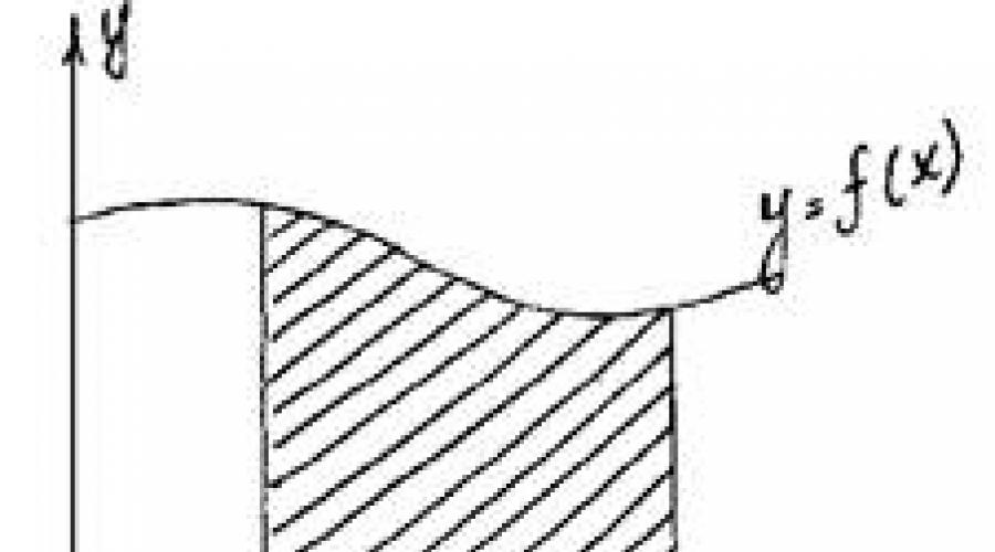
Using the exhaustion method and a number of other ingenious considerations (including the use of mechanics models), Archimedes solved many problems. He gave an estimate of the number p (3.10/71

Archimedes anticipated many of the ideas of integral calculus. (We add that in practice the first theorems on limits were proved by him.) But it took more than one and a half thousand years before these ideas found clear expression and were brought to the level of calculus.

Mathematicians of the 17th century, who obtained many new results, learned from the works of Archimedes. Another method was also actively used - the method of indivisibles, which also originated in Ancient Greece (it is associated primarily with the atomistic views of Democritus). For example, curvilinear trapezoid(Fig. 1, a) they imagined f(x) to be composed of vertical segments of length, to which they nevertheless attributed whether area equal to the infinitesimal value f(x). In accordance with this understanding, the required area was considered equal to the sum

an infinitely large number of infinitely small areas. Sometimes it was even emphasized that the individual terms in this sum are zeros, but zeros of a special kind, which, added to an infinite number, give a well-defined positive sum.

At least as it seems now dubious based on J. Kepler (1571-1630) in his writings “New Astronomy”.

Let it be necessary to find the area of the figure shown in Figure 1,b, where the curves bounding the figure above and below have the equations y = f(x) and y=f(x)+c.

Imagining a figure made up of “indivisible”, in Cavalieri’s terminology, infinitely thin columns, we notice that they all have a total length c. By moving them in the vertical direction, we can form them into a rectangle with base b-a and height c. Therefore, the required area is equal to the area of the resulting rectangle, i.e.

S = S1 = c (b – a).

Cavalieri's general principle for the areas of plane figures is formulated as follows: Let the lines of a certain pencil of parallels intersect the figures Ф1 and Ф2 along segments of equal length (Fig. 1c). Then the areas of the figures F1 and F2 are equal.

A similar principle operates in stereometry and is useful in finding volumes.

In the 17th century Many discoveries related to integral calculus were made. Thus, P. Fermat already in 1629 solved the problem of quadrature of any curve y = xn, where n is an integer (that is, he essentially derived the formula ò xndx = (1/n+1)xn+1), and on this basis solved a series of problems to find centers of gravity. I. Kepler, when deducing his famous laws of planetary motion, actually relied on the idea of approximate integration. I. Barrow (1630-1677), Newton's teacher, came close to understanding the connection between integration and differentiation. Work on representing functions in the form of power series was of great importance.

However, despite the significance of the results obtained by many extremely inventive mathematicians of the 17th century, calculus did not yet exist. It was necessary to highlight the general ideas underlying the solution of many particular problems, as well as to establish a connection between the operations of differentiation and integration, which gives a fairly general algorithm. This was done by Newton and Leibniz, who independently discovered a fact known as the Newton-Leibniz formula. Thus, the general method was finally formed. He still had to learn to find antiderivatives of many functions, give new logical calculus, etc. But the main thing had already been done: differential and integral calculus had been created.

Methods of mathematical analysis actively developed in the next century (first of all, the names of L. Euler, who completed a systematic study of the integration of elementary functions, and I. Bernoulli should be mentioned). Russian mathematicians M.V.Ostrogradsky (1801-1862), V.Ya.Bunyakovsky (1804-1889), P.L.Byshev (1821-1894) took part in the development of integral calculus. Of fundamental importance, in particular, were the results of Chebyshev, who proved that there are integrals that cannot be expressed through elementary functions.

A rigorous presentation of the integral theory appeared only in the last century. The solution to this problem is associated with the names of O. Cauchy, one of the greatest mathematicians, the German scientist B. Riemann (1826-1866), the French mathematician G. Darboux (1842-1917).

Answers to many questions related to the existence of areas and volumes of figures were obtained with the creation of the theory of measure by C. Jordan (1838-1922).

Various generalizations of the concept of integral already at the beginning of our century were proposed by the French mathematicians A. Lebesgue (1875-1941) and A. Denjoy (18 April 1974), with the Soviet mathematician A. Ya. inchinchin s (1894-1959).

Definition and properties of the integral

If F(x) is one of the antiderivatives of the function f(x) on the interval J, then the antiderivative on this interval has the form F(x)+C, where CОR.

Definition. The set of all antiderivatives of the function f(x) on the interval J is called the definite integral of the function f(x) on this interval and is denoted by òf(x)dx.

òf(x)dx = F(x)+C, where F(x) is some antiderivative on the interval J.

f – integrand function, f(x) – integrand expression, x – integration variable, C – integration constant.

Properties of the indefinite integral.

(òf(x)dx) ¢ = òf(x)dx ,

òf(x)dx = F(x)+C, where F¢(x) = f(x)

(òf(x)dx) ¢= (F(x)+C) ¢= f(x)

òf¢(x)dx = f(x)+C– from the definition.

ò k f (x)dx = k ò f¢(x)dx

if k is a constant and F¢(x)=f(x),

ò k f (x)dx = k F(x)dx = k(F(x)dx+C1)= k ò f¢(x)dx

ò (f(x)+g(x)+...+h(x))dx = ò f(x)dx + ò g(x)dx +...+ ò h(x)dx

ò (f(x)+g(x)+...+h(x))dx = ò dx =

= ò ¢dx = F(x)+G(x)+...+H(x)+C=

= òf(x)dx + òg(x)dx +...+ òh(x)dx, where C=C1+C2+C3+...+Cn.

Integration

Tabular method.

Substitution method.

If the integrand is not a table integral, then it is possible (not always) to apply this method. To do this you need:

split the integrand into two factors;

designate one of the factors of the new variable;

express the second factor through a new variable;

construct an integral, find its value and perform the reverse substitution.

Note: it is better to designate the new variable as the function that is associated with the remaining expression.

1. òxÖ(3x2–1)dx;

Let 3x2–1=t (t³0), take the derivative of both sides:

ódt 1 1 ó 1 1 t 2 2 1 ---Ø

ô- t 2 = - ô t 2dt = – --– + C = -Ö 3x2–1 +C

ò sin x cos 3x dx = ò – t3dt = – – + C

Let cos x = t

Method for converting an integrand into a sum or difference:

ò sin 3x cos x dx = 1/2 ò (sin 4x + sin 2x) dx = 1/8 cos 4x – ¼ cos 2x + C

ó x4+3x2+1 ó 1 1

ô---- dx = ô(x2+2 – --–) dx = - x2 + 2x – arctan x + C

Note: When solving this example, it is good to make polynomials by “angle”.

In parts

If it is impossible to take the integral in a given form, but at the same time, it is very easy to find the antiderivative of one factor and the derivative of another, then you can use the formula.

(u(x)v(x))’=u’(x)v(x)+u(x)v(x)

u’(x)v(x)=(u(x)v(x)+u(x)v’(x)

Let's integrate both sides

òu’(x)v(x)dx=ò (u(x)v(x))’dx – òu(x)v’(x)dx

ò u’(x)v(x)dx=u(x)v(x)dx – ò u(x)v’(x)dx

ò x cos (x) dx = ò x dsin x = x sin x – ò sin x dx = x sin x + cos x + C

Curvilinear trapezoid

Definition. A figure bounded by the graph of a continuous, constant-sign function f(x), the abscissa axis and the straight lines x=a, x=b is called a curvilinear trapezoid.

Methods for finding the area of a curved trapezoid

Theorem. If f(x) is a continuous and non-negative function on the segment , then the area of the corresponding curvilinear trapezoid is equal to the increment of the antiderivatives.

Given: f(x) – continuous indef. function, xО.

Prove: S = F(b) – F(a), where F(x) is the antiderivative of f(x).

Proof:

Let us prove that S(a) is an antiderivative of f(x).

D(f) = D(S) =

S’(x0)= lim(S(x0+Dx) – S(x0) / Dx), with Dx®0 DS – rectangle

Dx®0 with sides Dx and f(x0)

S’(x0) = lim(Dxf(x0) /Dx) = limf(x0)=f(x0): because x0 is a point, then S(x) –

Dx®0 Dx®0 is the antiderivative of f(x).

Therefore, by the theorem on the general form of the antiderivative, S(x)=F(x)+C.

Because S(a)=0, then S(a) = F(a)+C

S = S(b)=F(b)+C = F(b)–F(a)

The limit of this sum is called a definite integral.

The sum below the limit is called the integral sum.

A definite integral is the limit of the integral sum on an interval at n®¥. The integral sum is obtained as the limit of the sum of the products of the length of the segment obtained by dividing the domain of definition of the function at any point in this interval.

a is the lower limit of integration;

b - top.

Newton–Leibniz formula.

Comparing the formulas for the area of a curvilinear trapezoid, we conclude:

if F is an antiderivative for b on , then

ò f(x)dx = F(b)–F(a)

ò f(x)dx = F(x) ô = F(b) – F(a)

Properties of a definite integral.

ò f(x)dx = ò f(z)dz

ò f(x)dx = F(a) – F(a) = 0

ò f(x)dx = – ò f(x)dx

ò f(x)dx = F(a) – F(b) ò f(x)dx = F(b) – F(a) = – (F(a) – F(b))

If a, b and c are any points of the interval I on which the continuous function f(x) has an antiderivative, then

ò f(x)dx = ò f(x)dx + ò f(x)dx

F(b) – F(a) = F(c) – F(a) + F(b) – F(c) = F(b) – F(a)

(this is the additivity property of a definite integral)

If l and m are constant quantities, then

ò (lf(x) + mj(x))dx = lò f(x)dx + mòj(x))dx –

is the linearity property of a definite integral.

ò (f(x)+g(x)+...+h(x))dx = ò f(x)dx+ ò g(x)dx+...+ ò h(x)dx

ò (f(x)+g(x)+...+h(x))dx = (F(b) + G(b) +...+ H(b)) –

– (F(a) + G(a) +...+ H(a)) +C =

F(b)–F(a)+C1 +G(b)–G(a)+C2+...+H(b)–H(a)+Cn=

= ò f(x)dx+ ò g(x)dx+...+ ò h(x)dx

A set of standard pictures

S=ò f(x)dx + ò g(x)dx

Application of the integral

I. In physics.

Work of force (A=FScosa, cosa¹ 1)

If a force F acts on a particle, the kinetic energy does not remain constant. In this case, according to

the increment in the kinetic energy of a particle over time dt is equal to the scalar product Fds, where ds is the movement of the particle over time dt. Magnitude

is called the work done by force F.

Let the point move along the OX axis under the influence of a force, the projection of which on the OX axis is a function f(x) (f is a continuous function). Under the influence of force, the point moved from point S1(a) to S2(b). Let's divide the segment into n segments of the same length Dx = (b – a)/n. The work done by the force will be equal to the sum of the work done by the force on the resulting segments. Because f(x) is continuous, then for small the work done by the force on this segment is equal to f(a)(x1–a). Similarly, on the second segment f(x1)(x2–x1), on the nth segment - f(xn–1)(b–xn–1). Therefore the work is equal to:

A »An = f(a)Dx +f(x1)Dx+...+f(xn–1)Dx=

= ((b–a)/n)(f(a)+f(x1)+...+f(xn–1))

The approximate equality becomes exact as n®¥

A = lim [(b–a)/n] (f(a)+...+f(xn–1))= òf(x)dx (by definition)

Let a spring of stiffness C and length l be compressed to half its length. Determine the value of potential energy Ep equal to the work A performed by the force –F(s) the elasticity of the spring during its compression, then

Ep = A= – ò (–F(s)) dx

From the mechanics course it is known that F(s) = –Cs.

From here we find

Ep= – ò (–Cs)ds = CS2/2 | = C/2 l2/4

Answer: Cl2/8.

Center of mass coordinates

The center of mass is the point through which the resultant forces of gravity pass for any spatial arrangement of the body.

Let a material homogeneous plate o have the shape of a curvilinear trapezoid (x;y |a£x£b; 0£y£f(x)) and the function y=f(x) is continuous on , and the area of this curved trapezoid is equal to S, then the coordinates of the center The mass of the plate o is found using the formulas:

x0 = (1/S) ò x f(x) dx; y0 = (1/2S) ò f 2(x) dx;

Center of mass

Find the center of mass of a homogeneous semicircle of radius R.

Let's draw a semicircle in the OXY coordinate system.

y = (1/2S) òÖ(R2–x2)dx = (1/pR2) òÖ(R2–x2)dx =

= (1/pR2)(R2x–x3/3)|= 4R/3p

Answer: M(0; 4R/3p)

The path traveled by a material point

If a material point moves rectilinearly with speed u=u(t) and during the time T= t2–t1 (t2>t1) it has passed the path S, then

In geometry

Volume is a quantitative characteristic of a spatial body. A cube with an edge of 1 mm (1di, 1m, etc.) is taken as a unit of volume measurement.

The number of cubes of a unit volume placed in a given body is the volume of the body.

Axioms of volume:

Volume is a non-negative quantity.

The volume of a body is equal to the sum of the volumes of the bodies that make it up.

Let's find a formula for calculating volume:

choose the OX axis in the direction of the location of this body;

we will determine the boundaries of the location of the body relative to OX;

Let's introduce an auxiliary function S(x) that specifies the following correspondence: to each x from the segment we associate the cross-sectional area of this figure with a plane passing through a given point x perpendicular to the OX axis.

Let's divide the segment into n equal parts and through each point of the partition we draw a plane perpendicular to the OX axis, and our body will be divided into parts. According to the axiom

V=V1+V2+...+Vn=lim(S(x1)Dx +S(x2)Dx+...+S(xn)Dx

Dx®0, and Sk®Sk+1, and the volume of the part enclosed between two adjacent planes is equal to the volume of the cylinder Vc=SmainH.

We have the sum of the products of the function values at the partition points by the partition step, i.e. integral sum. By the definition of a definite integral, the limit of this sum as n®¥ is called the integral a

V= òS(x)dx, where S(x) is the section of the plane passing through

bselected point perpendicular to the OX axis.

To find the volume you need:

1). Select the OX axis in a convenient way.

2). Determine the boundaries of the location of this body relative to the axis.

3). Construct a section of this body with a plane perpendicular to the OX axis and passing through the corresponding point.

4). Express in terms of known quantities a function expressing the area of a given section.

5). Compose an integral.

6). After calculating the integral, find the volume.

Volume of rotation figures

A body obtained as a result of rotation of a flat figure relative to some axis is called a figure of rotation.

The function S(x) of the rotation figure is a circle.

Ssec(x)=p f 2(x)

Arc length of a plane curve

Let the function y = f(x) on the segment have a continuous derivative y’ = f ’(x). In this case, the arc length l of the “piece” of the graph of the function y = f(x), xО can be found using the formula

l = òÖ(1+f’(x)2)dx

Bibliography

M.Ya.Vilenkin, O.S.Ivashev-Musatov, S.I.Shvartsburd, “Algebra and mathematical analysis”, Moscow, 1993.

“Collection of problems on mathematical analysis”, Moscow, 1996.

I.V. Savelyev, “Course of General Physics”, volume 1, Moscow, 1982.

To view the presentation with pictures, design and slides, download its file and open it in PowerPoint on your computer.
Text content of presentation slides: The integral and its application in human life.
Goal: study and use of the integral in human activity. Objectives: find out what an integral is; identify all areas of human activity where the integral is used; find out what significance the integral has in human life. The scientist who created the integral. Eudoxus of Cnidus. Gave a complete proof of the theorem on the volume of a pyramid; theorems that the areas of two circles are related as the squares of their radii. In his proof, he used the so-called method of “exhausting” their radii. Two thousand years later, the method of “exhaustion” was transformed into the method of integration. What is an integral? Integral (from Latin Integer - whole) - an integral is the inverse of the differential of a function. Many physical and other problems come down to solving complex differential or integral equations. To do this, you need to know what differential and integral calculus are.𝑓𝑥𝑑𝑥 The symbol  was introduced by Gottfried Leibniz (1675). This sign is a modification of the Latin letter S (the first letter of the word summa). The word integral itself was coined by Jacob Bernoulli (1690). It comes from the Latin integro, which means to restore. J. BernoulliG. Leibniz Application of the integral. In geometry. Area of a plane figure. Definition: A figure bounded by the graph of a continuous, constant-sign function 𝑓(𝑥), the x-axis and straight lines 𝑥=𝑎, 𝑥=𝑏 is called a curvilinear trapezoid. Theorem. If 𝑓(𝑥) is a continuous and non-negative function on the segment [𝑎;𝑏], then the area of the corresponding curvilinear trapezoid is equal to the definite integral on this segment.𝑆 =𝑎𝑏𝑓𝑥𝑑𝑥= 𝐹(𝑏)–𝐹(𝑎) Volume of figures of rotation. The body obtained in The result of the rotation of the flat figure, relative to some axis, is called the rotation figure. Function 𝑆 (𝑥) 𝑓 (𝑥) rotation figures is a circle. In physics. Coordinates of the center of mass. The center of mass is the point through which the resultant force of gravity passes for any spatial location of the body. Let a material homogeneous plate have the shape of a curved trapezoid 𝑥;𝑦 𝑎≤𝑥≤𝑏; 0≤𝑦≤𝑓(𝑥)) and the function 𝑦=𝑓(𝑥) is continuous on [𝑎;𝑏], and the area of this curvilinear trapezoid is equal to 𝑆, then the coordinates of the center of mass of the plate o are found by the formulas:𝑥0 = 1𝑆 𝑎𝑏𝑥 𝑓( 𝑥 ) 𝑑𝑥; 𝑦0 = 12𝑆 𝑎𝑏𝑓 2(𝑥) 𝑑𝑥; Work done by force 𝐴=𝐹𝑆𝑐𝑜𝑠, 𝑐𝑜𝑠 1. If a force 𝐹 acts on a particle, the kinetic energy does not remain constant. In this case, according to 𝑑(𝑚2/2) = 𝐹𝑑𝑠, the increment in the kinetic energy of a particle over time dt is equal to the scalar product 𝐹𝑑𝑠, where 𝑑𝑠 is the movement of the particle over time 𝑑𝑡. The quantity𝑑𝐴=𝐹𝑑𝑠is called the work done by the force F.А = 𝑎𝑏𝑓𝑥𝑑𝑥 The path traveled by the material point. If the material point moves rectilinearly with speed 𝑣=𝑣(𝑡) and in time 𝑇= 𝑡2–𝑡1 ( 𝑡2>𝑡1) has passed the path 𝑆, then 𝑆 =𝑡1𝑡2𝑣(𝑡)𝑑𝑡. In economics, microeconomics courses often consider the so-called marginal values, i.e. for a given quantity, represented by some function 𝑦 =𝑓(𝑥), its derivative 𝑓′(𝑥) is considered. For example, if a cost function C is given depending on the volume q of the product produced 𝐶= 𝐶(𝑞), then the marginal costs will be given by the derivative of this function MC=С′(q). Its economic meaning is the cost of producing an additional unit of manufactured goods. Therefore, it is often necessary to find the cost function from a given marginal cost function. In biology, average flight length. We are interested in the average flight length. Since a circle is symmetrical with respect to any of its diameters, it is enough for us to limit ourselves to only those birds that fly in any one direction parallel to the Oy axis. Then the average span length is the average distance between the arcs ASV and 𝐴𝐶1𝐵. In other words, this is the average value of the function 𝑓1𝑥−𝑓2𝑥, where 𝑦=𝑓1𝑥 is the equation of the upper arc, and 𝑦=𝑓2𝑥 is the equation of the lower arc, i.e.𝐿=𝑎𝑏𝑓1𝑥−𝑓2𝑥𝑑𝑥𝑏− 𝑎 Since 𝑎𝑏𝑓1𝑥𝑑𝑥 equal to area curvilinear trapezoid аАСВb, 𝑎𝑏𝑓2𝑥𝑑𝑥 is equal to the area of the curvilinear trapezoid аА𝐶1Вb, then their difference is equal to the area of the circle, i.e. 𝜋𝑅2. The difference 𝑏−a is equal to 2R. Substituting this into 𝐿=𝑎𝑏𝑓1𝑥−𝑓2𝑥𝑑𝑥𝑏−𝑎 , we get: 𝐿=𝜋𝑅22𝑅=𝜋2𝑅

INTEGRAL. APPLICATION OF INTEGRALS.

Coursework in mathematics

Introduction

§1. History of integral calculus

The history of the concept of integral is closely connected with problems of finding quadratures. Mathematicians of Ancient Greece and Rome called problems on the quadrature of one or another flat figure to calculate areas. The Latin word quadratura translates as “to square.” The need for a special term is explained by the fact that in ancient times (and later, up to the 18th century), ideas about real numbers were not yet sufficiently developed. Mathematicians operated with their geometric analogues, or scalar quantities, which cannot be multiplied. Therefore, problems for finding areas had to be formulated, for example, like this: “Construct a square equal in size to the given circle.” (This classic problem “about squaring the circle”
circle" cannot, as is known, be solved using a compass and a ruler.)
The symbol o was introduced by Leibniz (1675). This sign is a modification of the Latin letter S (the first letter of the word summa). The word integral itself was coined by J. Bernulli (1690). It probably comes from the Latin integro, which translates as bringing to a previous state, restoring. (Indeed, the operation of integration “restores” the function by differentiating which the integrand was obtained.) Perhaps the origin of the term integral is different: the word integer means whole.
During the correspondence, I. Bernoulli and G. Leibniz agreed with J. Bernoulli’s proposal. At the same time, in 1696, the name of a new branch of mathematics appeared - integral calculus (calculus integralis), which was introduced by I. Bernoulli.
Other well-known terms related to integral calculus appeared much later. The name now in use, primitive function, replaced the earlier “primitive function,” which was introduced by Lagrange (1797). The Latin word primitivus is translated as “initial”: F(x) = o f(x)dx - initial (or original, or antiderivative) for f(x), which is obtained from F(x) by differentiation.
In modern literature, the set of all antiderivatives for the function f(x) is also called indefinite integral. This concept was highlighted by Leibniz, who noted that all antiderivative functions differ by an arbitrary constant.
b
A o f(x)dx
a
is called a definite integral (the designation was introduced by C. Fourier (1768-1830), but the limits of integration were already indicated by Euler).
Many significant achievements of mathematicians of Ancient Greece in solving problems of finding quadratures (i.e., calculating areas) of plane figures, as well as cubatures (calculating volumes) of bodies are associated with the use of the exhaustion method proposed by Eudoxus of Cnidus (c. 408 - c. 355 BC .e.). Using this method, Eudoxus proved, for example, that the areas of two circles are related as the squares of their diameters, and the volume of a cone is equal to 1/3 of the volume of a cylinder having the same base and height.
Eudoxus' method was improved by Archimedes. The main stages characterizing Archimedes' method: 1) it is proved that the area of a circle is less than the area of any regular polygon described around it, but greater than the area of any inscribed; 2) it is proved that with an unlimited doubling of the number of sides, the difference in the areas of these polygons tends to zero; 3) to calculate the area of a circle, it remains to find the value to which the ratio of the area of a regular polygon tends when the number of its sides is unlimitedly doubled.
Using the exhaustion method and a number of other ingenious considerations (including the use of mechanics models), Archimedes solved many problems. He gave an estimate of the number p (3.10/71 Archimedes anticipated many of the ideas of integral calculus. (We add that in practice the first theorems on limits were proved by him.) But it took more than one and a half thousand years before these ideas found clear expression and were brought to the level of calculus.
Mathematicians of the 17th century, who obtained many new results, learned from the works of Archimedes. Another method was also actively used - the method of indivisibles, which also originated in Ancient Greece (it is associated primarily with the atomistic views of Democritus). For example, they imagined a curved trapezoid (Fig. 1, a) to be composed of vertical segments of length f(x), to which they nevertheless assigned an area equal to the infinitesimal value f(x)dx. In accordance with this understanding, the required area was considered equal to the sum
S = a f(x)dx
a an infinitely large number of infinitely small areas. Sometimes it was even emphasized that the individual terms in this sum are zeros, but zeros of a special kind, which, added to an infinite number, give a well-defined positive sum.
On such a now seemingly at least dubious basis, J. Kepler (1571-1630) in his writings “New Astronomy”.

(1609) and “Stereometry of wine barrels” (1615) correctly calculated a number of areas (for example, the area of a figure bounded by an ellipse) and volumes (the body was cut into 6 finitely thin plates). These studies were continued by the Italian mathematicians B. Cavalieri (1598-1647) and E. Torricelli (1608-1647). The principle formulated by B. Cavalieri, introduced by him under some additional assumptions, retains its significance in our time.
Let it be necessary to find the area of the figure shown in Figure 1,b, where the curves bounding the figure above and below have the equations y = f(x) and y=f(x)+c.
Imagining a figure made up of “indivisible”, in Cavalieri’s terminology, infinitely thin columns, we notice that they all have a total length c. By moving them in the vertical direction, we can form them into a rectangle with base b-a and height c. Therefore, the required area is equal to the area of the resulting rectangle, i.e.
S = S 1 = c (b – a).
Cavalieri's general principle for the areas of plane figures is formulated as follows: Let the lines of a certain pencil of parallel intersect the figures Ф 1 and Ф 2 along segments of equal length (Fig. 1, c). Then the areas of the figures Ф 1 and Ф 2 are equal.
A similar principle operates in stereometry and is useful in finding volumes.
In the 17th century Many discoveries related to integral calculus were made. Thus, P. Fermat already in 1629 solved the problem of quadrature of any curve y = x n, where n is an integer (that is, he essentially derived the formula o x n dx = (1/n+1)x n+1), and On this basis, I solved a number of problems on finding centers of gravity. I. Kepler, when deducing his famous laws of planetary motion, actually relied on the idea of approximate integration. I. Barrow (1630-1677), Newton's teacher, came close to understanding the connection between integration and differentiation. Work on representing functions in the form of power series was of great importance.
However, despite the significance of the results obtained by many extremely inventive mathematicians of the 17th century, calculus did not yet exist. It was necessary to highlight the general ideas underlying the solution of many particular problems, as well as to establish a connection between the operations of differentiation and integration, which gives a fairly general algorithm. This was done by Newton and Leibniz, who independently discovered a fact known as the Newton-Leibniz formula. Thus, the general method was finally formed. He still had to learn to find antiderivatives of many functions, give new logical calculus, etc. But the main thing had already been done: differential and integral calculus had been created.
Methods of mathematical analysis actively developed in the next century (first of all, the names of L. Euler, who completed a systematic study of the integration of elementary functions, and I. Bernoulli should be mentioned). Russian mathematicians M.V. Ostrogradsky (1801-1862), V.Ya. Bunyakovsky (1804-1889), P.L. Chebyshev (1821-1894) took part in the development of integral calculus. Of fundamental importance, in particular, were the results of Chebyshev, who proved that there are integrals that cannot be expressed through elementary functions.
A rigorous presentation of the integral theory appeared only in the last century. The solution to this problem is associated with the names of O. Cauchy, one of the greatest mathematicians, the German scientist B. Riemann (1826-1866), the French mathematician G. Darboux (1842-1917).
Answers to many questions related to the existence of areas and volumes of figures were obtained with the creation of the theory of measure by C. Jordan (1838-1922).
Various generalizations of the concept of integral were proposed already at the beginning of this century by the French mathematicians A. Lebesgue (1875-1941) and A. Denjoy (1884-1974), and the Soviet mathematician A. Ya. Khinchinchin (1894-1959).

§2. Definition and properties of the integral

If F(x) is one of the antiderivatives of the function f(x) on the interval J, then the antiderivative on this interval has the form F(x)+C, where CIR.
Definition. The set of all antiderivatives of the function f(x) on the interval J is called the definite integral of the function f(x) on this interval and is denoted by o f(x)dx.
o f(x)dx = F(x)+C, where F(x) is some antiderivative on the interval J.
f – integrand function, f(x) – integrand expression, x – integration variable, C – integration constant.

Properties of the indefinite integral

o f(x)dx = F(x)+C, where F ?(x) = f(x)
(o f(x)dx) ?= (F(x)+C) ?= f(x)

if k is a constant and F ?(x)=f(x),
o k f (x)dx = k F(x)dx = k(F(x)dx+C 1)= k o f?(x)dx

o (f(x)+g(x)+...+h(x))dx = o dx =
= o ?dx = F(x)+G(x)+...+H(x)+C=
= o f(x)dx + o g(x)dx +...+ o h(x)dx, where C=C 1 +C 2 +C 3 +...+C n.

Integration

If the integrand is not a table integral, then it is possible (not always) to apply this method. To do this you need:

Note: it is better to designate the new variable as the function that is associated with the remaining expression.

Examples:
1.
Let 3x 2 –1=t (t?0), take the derivative of both sides:
6xdx = dt
xdx=dt/6

2.
o sin x cos 3 x dx = o – t 3 dt = + C
Let cos x = t
-sin x dx = dt

Examples:

o x 4 +3x 2 +1 o 1 1
o---- dx = o(x 2 +2 – --–) dx = - x 2 + 2x – arctan x + C
o x 2 +1 o x 2 +1 3

Note: When solving this example, it is good to make polynomials by “angle”.

If it is impossible to take the integral in a given form, but at the same time, it is very easy to find the antiderivative of one factor and the derivative of another, then you can use the formula.
(u(x)v(x))’=u’(x)v(x)+u(x)v(x)
u’(x)v(x)=(u(x)v(x)+u(x)v’(x)
Let's integrate both sides
o u’(x)v(x)dx=o (u(x)v(x))’dx – o u(x)v’(x)dx
o u’(x)v(x)dx=u(x)v(x)dx – o u(x)v’(x)dx

Example:

x = u(x)cos x = v’(x)

§3. Curvilinear trapezoid

Definition. A figure bounded by the graph of a continuous, constant-sign function f(x), the abscissa axis and the straight lines x=a, x=b is called a curvilinear trapezoid.

Methods for finding the area of a curved trapezoid

Given: f(x) – continuous indef. function, xI.
Prove: S = F(b) – F(a), where F(x) is the antiderivative of f(x).
Proof:

D x ® 0 with sides Dx and f(x 0)
S’(x 0) = lim(Dx f(x 0) /Dx) = lim f(x 0)=f(x 0): because x0 is a point, then S(x) –
D x ® 0 D x ® 0 antiderivative f(x).
Therefore, by the theorem on the general form of the antiderivative, S(x)=F(x)+C.

C = –Fa

II.

The limit of this sum is called a definite integral.
b
S tr =o f(x)dx
a
The sum below the limit is called the integral sum.
A definite integral is the limit of the integral sum on an interval at n®?. The integral sum is obtained as the limit of the sum of the products of the length of the segment obtained by dividing the domain of definition of the function at any point in this interval.
a is the lower limit of integration;
b - top.

Newton–Leibniz formula

Comparing the formulas for the area of a curvilinear trapezoid, we conclude:
if F is an antiderivative for b on , then
b
o f(x)dx = F(b)–F(a)
a
b b
o f(x)dx = F(x) o = F(b) – F(a)
a a

§4. A set of standard pictures

b b
S=o f(x)dx + o g(x)dx
a a

§5. Application of the integral

I. In physics

Work of force (A=FScosa, cosa ? 1)

If a force F acts on a particle, the kinetic energy does not remain constant. In this case, according to
d(mu 2 /2) = Fds
the increment in the kinetic energy of a particle over time dt is equal to the scalar product Fds, where ds is the movement of the particle over time dt. Magnitude
dA=Fds
is called the work done by force F.

Let the point move along the OX axis under the influence of a force, the projection of which on the OX axis is a function f(x) (f is a continuous function). Under the influence of force, the point moved from point S 1 (a) to S 2 (b). Let's divide the segment into n segments of the same length Dx = (b – a)/n. The work done by the force will be equal to the sum of the work done by the force on the resulting segments. Because f(x) is continuous, then for small the work done by the force on this segment is equal to f(a)(x 1 –a). Similarly, on the second segment f(x 1)(x 2 –x 1), on the nth segment - f(x n–1)(b–x n–1). Therefore the work is equal to:

A » A n = f(a)Dx +f(x 1)Dx+...+f(x n–1)Dx=
= ((b–a)/n)(f(a)+f(x 1)+...+f(x n– 1))
The approximate equality becomes exact at n®?
b
A = lim [(b–a)/n] (f(a)+...+f(x n–1))= o f(x)dx (by definition)
n®? a

Example 1:
Let a spring of stiffness C and length l be compressed to half its length. Determine the value of potential energy Ep equal to the work A performed by the force –F(s) the elasticity of the spring during its compression, then
l/2
E p = A= – o (–F(s)) dx
0
From the mechanics course it is known that F(s) = –Cs.
From here we find
l/2 l/2
E p = – o (–Cs)ds = CS 2 /2 | = C/2 l 2 /4
0 0
Answer: Cl 2 /8.

Example 2:
How much work must be done to stretch the spring by 4 cm, if it is known that under a load of 1 N it stretches by 1 cm?
Solution:
According to Hooke's law, the force X N, stretching the spring by x, is equal to X = kx. We find the proportionality coefficient k from the condition: if x = 0.01 m, then X = 1 N, therefore, k = 1/0.01 = 100 and X = 100x. Then
(J)
Answer: A=0.08 J

Example 3:
Using a crane, a reinforced concrete hollow is removed from the bottom of a river 5 m deep. What work will be done if the hollow has the shape of a regular tetrahedron with an edge of 1 m? The density of reinforced concrete is 2500 kg/m3, the density of water is 1000 kg/m3.
Solution:
y
0

The height of the tetrahedron is m, the volume of the tetrahedron is m 3. The weight of the hole in water, taking into account the action of the Archimedean force, is equal to
(J).
Now let’s find the work A i when removing the gouge from the water. Let the vertex of the tetrahedron reach a height of 5+y, then the volume of the small tetrahedron emerging from the water is equal, and the weight of the tetrahedron is:
.
Hence,

(J).
Hence A=A 0 +A 1 =7227.5 J + 2082.5 J = 9310 J = 9.31 kJ
Answer: A=9.31 (J).

Example 4:
What pressure force does a rectangular plate of length a and width b (a>b) experience if it is inclined to the horizontal surface of the liquid at an angle? and its larger side is at depth h?

Answer: P= .

Center of mass coordinates

The center of mass is the point through which the resultant forces of gravity pass for any spatial arrangement of the body.
Let a material homogeneous plate o have the shape of a curved trapezoid (x;y |a?x?b; 0?y?f(x)) and the function y=f(x) is continuous on , and the area of this curved trapezoid is equal to S, then the coordinates of the center The mass of the plate o is found using the formulas:
b b
x 0 = (1/S) o x f(x) dx; y 0 = (1/2S) o f 2 (x) dx;
a a

Example 1:
Find the center of mass of a homogeneous semicircle of radius R.
Let's draw a semicircle in the OXY coordinate system.

R R
y = (1/2S) oO(R 2 –x 2)dx = (1/pR 2) oO(R 2 –x 2)dx =
–R –R
R
= (1/pR 2)(R 2 x–x 3 /3)|= 4R/3p
–R
Answer: M(0; 4R/3p).

Example 2:
Find the coordinates of the center of gravity of the figure bounded by the ellipse arc x=acost, y=bsint, located in the first quarter, and the coordinate axes.
Solution:
In the first quarter, as x increases from 0 to a, the value of t decreases from?/2 to 0, therefore

Using the formula for the area of the ellipse S=?ab, we get

The path traveled by a material point
If a material point moves rectilinearly with speed u=u(t) and during the time T= t 2 –t 1 (t 2 >t 1) it has passed the path S, then
t2
S = o u(t)dt.
t 1

Volume is a quantitative characteristic of a spatial body. A cube with an edge of 1 mm (1 dm, 1 m, etc.) is taken as a unit of volume measurement.
The number of cubes of a unit volume placed in a given body is the volume of the body.

Axioms of volume:

Let's find a formula for calculating volume:

V=V 1 +V 2 +...+V n =lim(S(x1)Dx +S(x2)Dx+...+S(xn)Dx
n®?
Dx®0, and S k ®S k+1, and the volume of the part enclosed between two adjacent planes is equal to the volume of the cylinder V c =S main H.
We have the sum of the products of the function values at the partition points by the partition step, i.e. integral sum. By the definition of a definite integral, the limit of this sum for n®? called integral

A
V = o S(x)dx, where S(x) is the section of the plane passing through
b selected point perpendicular to the OX axis.

To find the volume you need:
1) Select the OX axis in a convenient way.
2) Determine the boundaries of the location of this body relative to the axis.
3) Construct a section of this body with a plane perpendicular to the OX axis and passing through the corresponding point.
4) Express through known quantities a function expressing the area of a given section.
5) Compose an integral.
6) After calculating the integral, find the volume.

Example 1:
Find the volume of a triaxial ellipse.

Solution:
Plane sections of an ellipsoid parallel to the xOz plane and spaced from it at a distance y=h represent an ellipse

With axle shafts and...
Let's find the area of this section
.
Let's find the volume of the ellipse:

Example 2:
Find the volume of a body whose base is an isosceles triangle with height h and base a. The cross section of a body is a segment of a parabola with a chord equal to the height of the segment.

Solution:
We have, Let us express the cross-sectional area as a function of z, for which we first find the equation of the parabola. The length of the chord DE can be found from the similarity of the corresponding triangles, namely:
those. . Let us assume that then the equation of the parabola in the uKv coordinate system will take the form. From here we find the cross-sectional area of this body:
or.
Thus, .
Answer:
Volume of rotation figures

A body obtained as a result of rotation of a flat figure relative to some axis is called a figure of rotation.
The function S(x) of the rotation figure is a circle.
S sech = pr 2
S sec (x)=p f 2 (x)

Arc length of a plane curve

Let the function y = f(x) on the segment have a continuous derivative y’ = f’(x). In this case, the arc length l of the “piece” of the graph of the function y = f(x), xI can be found using the formula:

Example 1:
Find the arc length of the curve from x=0 to x=1 (y?0)
Solution:
Differentiating the equation of the curve, we find. Thus,
.
Answer: .

Conclusion
The integral is used in sciences such as physics, geometry, mathematics and other sciences. Using the integral, the work of the force is calculated, the coordinates of the center of mass and the path traveled by the material point are found. In geometry it is used to calculate the volume of a body, find the arc length of a curve, etc.
Literature

The concept of integral is widely applicable in life. Integrals are used in various fields of science and technology. The main problems calculated using integrals are problems on:

1. Finding the volume of a body

2. Finding the center of mass of the body.

Let's look at each of them in more detail. Here and below, to denote the definite integral of some function f(x), with the limits of integration from a to b, we will use the following notation ∫ a b f(x).

Finding the volume of a body

Consider the following figure. Suppose there is a certain body whose volume is equal to V. There is also a straight line such that if we take a certain plane perpendicular to this straight line, the cross-sectional area S of this body by this plane will not be known.

Each such plane will be perpendicular to the Ox axis, and therefore will intersect it at some point x. That is, each point x from the segment will be assigned a number S(x) - the cross-sectional area of the body, the plane passing through this point.

It turns out that some function S(x) will be specified on the segment. If this function is continuous on this segment, then the following formula will be valid:

V = ∫ a b S(x)dx.

The proof of this statement goes beyond the school curriculum.

Calculation of the body's center of mass

Center of mass is most often used in physics. For example, there is a body that moves at a certain speed. But it is inconvenient to consider a large body, and therefore in physics this body is considered as the movement of a point, under the assumption that this point has the same mass as the whole body.

And the task of calculating the center of mass of the body is the main one in this matter. Because the body is large, and what point exactly should be taken as the center of mass? Maybe the one in the middle of the body? Or maybe the point closest to the front edge? This is where integration comes to the rescue.

To find the center of mass, the following two rules are used:

1. The x’ coordinate of the center of mass of a certain system of material points A1, A2, A3, … An with masses m1, m2, m3, … mn, respectively located on a straight line at points with coordinates x1, x2, x3, … xn is found by the following formula:

x’ = (m1*x1 + ma*x2 + … + mn*xn)/(m1 + m2 + m3 +… + mn)

2. When calculating the coordinates of the center of mass, you can replace any part of the figure in question with a material point, placing it at the center of mass of this separate part of the figure, and taking the mass equal to the mass of this part of the figure.

For example, if a mass with density p(x) is distributed along a rod - a segment of the Ox axis, where p(x) is a continuous function, then the coordinate of the center of mass x' will be equal to.